Selective G-Bispectrum

Invariance is the easy part. You can always take an average or a max over a group and call it a day.

The hard part is being invariant without throwing away the signal.

This article is about a specific fix: the Selective $G$ -Bispectrum, introduced in the NeurIPS 2024 paper The Selective $G$ -Bispectrum and its Inversion: Applications to $G$ -Invariant Networks (in this repo under papers/bispectrum/).

The problem: “invariant” can mean “information-destroying”

Group-equivariant CNNs ( $G$ -CNNs) are great at carrying symmetries through layers. But at some point (classification, retrieval, etc.) you usually want $G$ -invariance: rotate the input, same answer.

The default invariant layer is $G$ -pooling:

Avg $G$ -pooling: $\Theta \mapsto \frac{1}{|G|}\sum_{g\in G}\Theta(g)$
Max $G$ -pooling: $\Theta \mapsto \max_{g\in G}\Theta(g)$

Both are invariant, and both are cheap. But they can erase structure so aggressively that two inputs that are not related by a group action can map to the same pooled value.

Max pooling is a “bag of features” approach. It knows a feature exists somewhere, but forgets where it is relative to other features. It can’t distinguish a face from a Picasso painting where the eye is on the chin.

This also explains why max pooling sometimes works: if you have enough filters, a giant bag-of-features can approximate structure indirectly. But it’s a crude contract: you buy invariance by destroying geometry, and then you buy geometry back with width.

The money shot: parameter efficiency (why engineers should care)

The paper’s strongest practical argument isn’t just “invariance.” It’s parameter efficiency.

Because max pooling throws away relative structure, you often need to compensate with a wider $G$ -convolution (more filters). The Selective $G$ -Bispectrum layer is structure-preserving, so it stays strong under tight filter budgets.

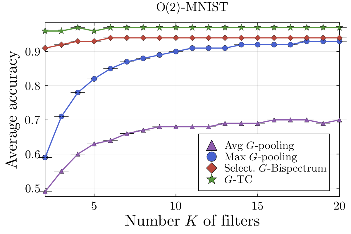
In the paper’s MNIST experiments, the effect is dramatic: with only $K=2$ filters, the Selective $G$ -Bispectrum stays around ~95% accuracy while max pooling can drop to ~60%, and max pooling only catches up once you throw enough filters at it.

Accuracy vs number of filters for O(2)-MNIST (dihedral discretization), comparing avg/max pooling, Selective G-Bispectrum, and G-TC. — Figure 1. Parameter efficiency: max pooling is a lossy bottleneck, so you need width to compensate. The Selective $G$-Bispectrum preserves structure, so it stays accurate even with a small filter budget. PDF

The alternative: complete $G$ -invariants (TC / bispectrum)

There’s a stronger notion than “invariant” that matters in practice:

A complete $G$ -invariant is one where (generically) equal outputs imply equal inputs up to group action.

In the paper’s framing, the $G$ -Triple Correlation ( $G$ -TC) and the full $G$ -Bispectrum have this property under mild “genericity” assumptions on the Fourier coefficients.

⁺

The “genericity” assumption is basically “no accidental singularities / zeros,” i.e. corner cases of measure zero; small perturbations usually fix it.

This is exactly what you want from a pooling-like primitive if you care about robustness: it removes only the nuisance symmetry, not the content.

The blocker: cost explodes with $|G|$

Completeness has historically been expensive:

$G$ -TC: $\mathcal{O}(|G|^2)$ outputs and $\mathcal{O}(|G|^3)$ compute (per feature map, roughly).
Full $G$ -bispectrum: $\mathcal{O}(|G|^2)$ outputs and $\mathcal{O}(|G|^2)$ compute.
Pooling: $\mathcal{O}(1)$ outputs and $\mathcal{O}(|G|)$ compute.

So the practical choice was often: “cheap and lossy” vs “complete and prohibitive.”

The core idea: bispectrum redundancy → selective bispectrum

The paper’s main observation is that the full $G$ -bispectrum contains redundancy. The non-magic intuition is generating sets: just as a group can be generated by a small set of elements, the spectral information can be recovered from a small chain of bispectral “links.” You don’t need every pair $(\rho_1,\rho_2)$ ; you need enough pairs to traverse the graph of representations induced by tensor products (Kronecker decompositions) and reconstruct everything up to the inherent group-action ambiguity.

That subset is the Selective $G$ -Bispectrum:

Space (linear): $\mathcal{O}(|G|)$ coefficients (instead of $\mathcal{O}(|G|^2)$ ).
Time: near-linear $\mathcal{O}(|G|\log |G|)$ if a fast Fourier transform exists for the group; otherwise it’s quadratic $\mathcal{O}(|G|^2)$ (still far better than the cubic $G$ -TC).
Completeness: proved for the big practical families (finite commutative groups, dihedral groups, octahedral / full octahedral groups).

The hidden cost of completeness (you can’t just import this)

If you are used to PyTorch’s nn.MaxPool, you are spoiled. Max pooling is stateless and agnostic: it doesn’t care about the mathematical properties of the data it crushes. It just looks for the highest number and moves on.

The Selective $G$ -Bispectrum is not a drop-in, stateless replacement. It is structure-aware, and that structure requires a strict setup cost.

The mechanism: routing tables for symmetry

Unlike standard pooling (spatial pixels), the $G$ -bispectrum operates in the spectral domain.

At a high level the layer has a preamble:

$G$ -Fourier transform: the feature map $\Theta$ is mapped to Fourier blocks indexed by irreps $\rho$ , i.e. $\hat{\Theta}(\rho)$ .
Tensor contraction: those blocks are combined using the bispectrum formula, which includes Clebsch–Gordan / Kronecker structure telling you how frequency modes mix under tensor products.

The “selective” part is where the paper gets clever: it consults a Kronecker table (think: a routing map over irreps) and computes only a sparse chain of interactions—enough to traverse the representation graph and preserve completeness—rather than filling the entire $\mathcal{O}(|G|^2)$ grid.

Kronecker tables for D4 and an octahedral group, highlighting the sparse coefficient pairs used by the Selective G-Bispectrum compared to the full grid. — Figure 3. Routing for completeness: the full bispectrum is the full irrep-pair grid; the Selective $G$-Bispectrum is a sparse path through it chosen to preserve invertibility up to group action. PDF

The implementation gap (the precomputed constants)

Because this layer depends on group structure, you aren’t just passing a tensor; you’re passing it through a gauntlet of precomputed representation-theoretic constants:

The hard way: manually compute irreps, Clebsch–Gordan matrices, Kronecker decompositions for your group, cache them, and write the sparse contractions efficiently.
The smart way: lean on geometric deep learning libraries (the paper’s code builds on escnn) to generate irreps / transformation structure and to manage the bookkeeping.

The FFT caveat (software maturity, not theory)

The theoretical “fast” scaling ( $\mathcal{O}(|G|\log |G|)$ ) relies on the existence of a fast Fourier transform for your group.

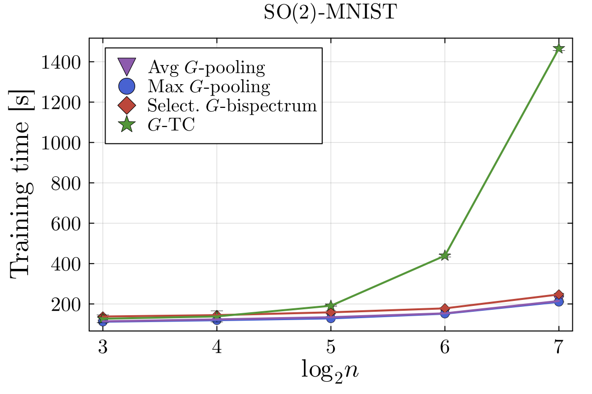
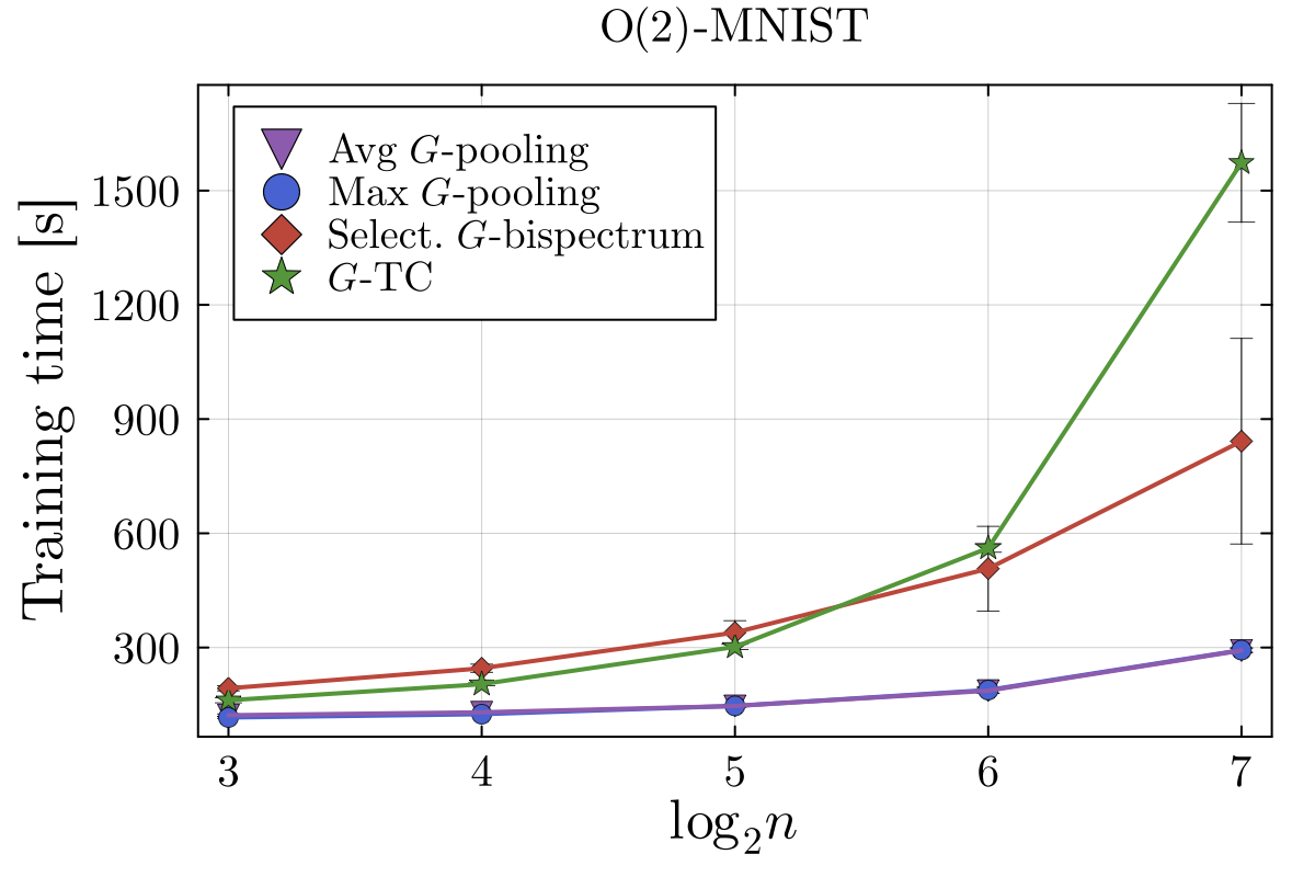
For groups where we rely on classical DFTs (including typical dihedral implementations in practice), compute scales quadratically: $\mathcal{O}(|G|^2)$ . That’s still significantly faster than the cubic $G$ -TC, but it’s not “instant” until dihedral FFT plumbing is real.

A small table of the tradeoffs

Invariant layer	Time (per feature map, rough)	Output size	Complete $G$ -invariant
Avg/Max $G$ -pooling	$\mathcal{O}(\lvert G\rvert)$	$\mathcal{O}(1)$	No
$G$ -TC	$\mathcal{O}(\lvert G\rvert^3)$	$\mathcal{O}(\lvert G\rvert^2)$	Yes
Full $G$ -bispectrum	$\mathcal{O}(\lvert G\rvert^2)$	$\mathcal{O}(\lvert G\rvert^2)$	Yes
Selective $G$ -Bispectrum	$\mathcal{O}(\lvert G\rvert\log\lvert G\rvert)$ if FFT else $\mathcal{O}(\lvert G\rvert^2)$	$\mathcal{O}(\lvert G\rvert)$	Yes

What it looks like as a layer

Architecturally, it’s “swap the invariant module” after a $G$ -convolution: same $G$ -conv backbone, different bottleneck.

Implementation note (the catch)

This is not nn.MaxPool. Computing $G$ -bispectral coefficients involves the group Fourier transform and Clebsch–Gordan / Kronecker structure (e.g. precomputed Kronecker tables, Clebsch–Gordan matrices). In practice you lean on libraries like escnn, or you precompute the representation-theoretic pieces once for your group and reuse them.

Diagram of a G-CNN: input → G-convolution → invariant layer choice (max pooling, G-TC, selective/full G-bispectrum) → secondary network. — Figure 4. G-CNN architecture: the Selective $G$-Bispectrum replaces pooling as a structure-preserving bottleneck. PDF

Empirics: the regime where it matters

The experiments (MNIST / EMNIST under discrete rotation and rotation+reflection groups) are pretty consistent with the theory:

Speed: with FFTs (cyclic groups), selective bispectrum scales close to linearly in $|G|$ , while $G$ -TC scales cubically.
Accuracy: selective bispectrum is typically much better than max/avg pooling when you don’t have a huge filter budget.
Tradeoff: $G$ -TC can still win slightly on accuracy (even though both are complete in theory), plausibly because redundancy makes the downstream MLP’s job easier at finite width.

Training time scaling plot for cyclic groups C_n comparing invariant layers (avg/max pooling, selective G-bispectrum, G-TC). — Figure 5. With an FFT on C_n, selective bispectrum tracks pooling-like scaling while retaining completeness; G-TC becomes the bottleneck as |G| grows. PDF

Training time scaling plot for dihedral groups D_n comparing invariant layers. — Figure 6. Reality check: for $D_n$, many current implementations rely on a classical DFT, so selective bispectrum scales quadratically. It’s still dramatically better than cubic $G$-TC, but it’s not “instant” until a dihedral FFT is in place. PDF

Takeaway (the “why this matters” sentence)

Max pooling buys invariance at the cost of signal destruction, forcing you to compensate with wider networks. The Selective $G$ -Bispectrum offers a new contract: complete signal preservation at linear space cost. It lets models be invariant and parameter-efficient, making it the first credible “complete” default for realistic $G$ -CNN pipelines.