Implementing the Selective G-Bispectrum

You can’t just import this.

If you are used to PyTorch’s nn.MaxPool, you are spoiled. Max pooling is stateless and agnostic; it doesn’t care about the mathematical properties of the data it crushes. It just looks for the highest number and moves on.

The Selective $G$ -Bispectrum is not that. It is structure-aware, and that structure creates a one-time setup tax you pay to make runtime cheap.

This article is the implementation view: what’s actually in the layer, what you precompute, and what a practical codebase needs to cache.

What the layer is doing (in the only order that matters: runtime order)

Assume you already have a $G$ -CNN backbone that produces a feature map $\Theta:G\to\mathbb{R}$ (per filter, per channel, etc.). The Selective $G$ -Bispectrum layer computes a structure-preserving invariant summary of that $\Theta$ .

At runtime, the pipeline is:

$G$ -Fourier transform: map $\Theta$ to Fourier blocks indexed by irreps $\rho$ (think: $\hat{\Theta}(\rho)$ , often a matrix per irrep).
Bispectral contraction: combine irrep blocks according to the bispectrum formula.
Select only a sparse set of irrep pairs: instead of all $(\rho_1,\rho_2)$ pairs, compute only those dictated by the selection procedure (the “routing table”).

The key is that step (3) can be sparse without losing completeness (up to group action), for the major finite groups used in practice.

The mechanism: routing tables over representations

The “selective” part is not magic. It’s closer to graph traversal.

Tensor products of irreps decompose into direct sums. The paper represents this bookkeeping via a Kronecker table (you can read it as an adjacency structure: which irrep pairs can “reach” which other irreps via tensor-product mixing).

Instead of computing the full irrep-pair grid (full bispectrum), the Selective $G$ -Bispectrum computes a sparse chain of bispectral coefficients chosen to traverse that representation graph—analogous to generating a group from a small generating set.

Kronecker tables for D4 and an octahedral group, with selected coefficient pairs highlighted for the Selective G-Bispectrum. — Figure 1. Routing for completeness: the colored cells are the sparse irrep pairs the Selective $G$-Bispectrum keeps. The uncolored grid is the quadratic redundancy you avoid. PDF

The precompute tax (the stuff pooling never makes you think about)

1) Irreps + Fourier transform implementation

To compute $\hat{\Theta}(\rho)$ you need a concrete $G$ -Fourier transform implementation for your group (or a library that provides it).

For many groups, the “fast” story depends on specialized FFTs. Without them, you’re in DFT land (dense linear algebra).

2) Clebsch–Gordan / Kronecker structure

On groups, “multiplying frequencies” is not scalar multiplication; it’s representation mixing. That mixing is governed by Clebsch–Gordan (CG) coefficients (or equivalently CG matrices / change-of-basis maps) and the decomposition of tensor products.

In other words: the bispectrum layer is not just a reduction; it’s a contraction against a pile of group-specific constants.

⁺

This is the point where most “drop-in layer” mental models die. The layer needs group-specific algebra baked in.

3) The selection itself (which pairs to compute)

You need the selection list of irrep pairs (the sparse “routing plan”). For different groups, the chosen sequence differs, because the tensor-product graph differs.

The paper provides a general selection procedure and then proves completeness for the major group families it cares about.

Selective G-Bispectrum algorithm illustration showing how selected coefficients are added based on Kronecker decomposition structure. — Figure 2. One way to read the algorithm: keep adding coefficient pairs that let you reach irreps you couldn’t reach before, until you can traverse the full set. PDF

The implementation gap: what a real PyTorch project does

There is no torch.signal.selective_bispectrum.

So you choose:

Hard way: implement the group’s irreps + CG machinery yourself, cache it, and write the sparse contractions efficiently (likely custom kernels if you care about performance).
Smart way: lean on existing geometric deep learning libraries (the paper’s implementation builds on escnn) to generate irreps / group actions and handle representation bookkeeping.

Either way, if you want this layer to be fast in training, you end up caring about:

Caching: CG matrices, decomposition metadata, irrep indexing, selection lists (these should be constructed once, then reused).
Memory layout: you want contraction-friendly layouts so the “sparse list of pairs” doesn’t become a scatter/gather disaster.
Numerics: “complete in theory” still assumes genericity; corner-case singularities are real in finite precision.

FFT caveat: theory vs what you can run today

The headline speed ( $\mathcal{O}(\lvert G\rvert\log\lvert G\rvert)$ ) is conditional: it assumes an FFT exists for your group and your code actually uses it.

For cyclic groups $C_n$ , FFTs are mature and the layer can be close to pooling-like scaling.

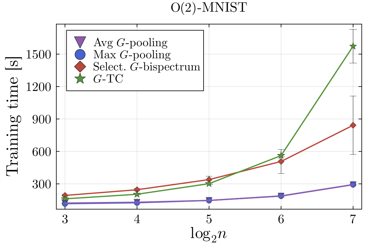
For dihedral groups $D_n$ (the common “rotations + flips” workhorse for 2D images), many implementations fall back to classical DFTs, pushing compute toward $\mathcal{O}(\lvert G\rvert^2)$ . Still way better than cubic $G$ -TC—but you should think of it as “quadratic but complete,” not “free.”

Training time scaling plot for dihedral groups D_n comparing invariant layers. — Figure 3. Implementation reality: without a dihedral FFT, selective bispectrum scales quadratically. That’s still a huge win over cubic $G$-TC. PDF

Bottom line

Max pooling buys invariance by destroying structure, then you buy structure back with width.

The Selective $G$ -Bispectrum buys invariance with a different contract: pay a setup tax (group constants + routing), then get a layer that is mathematically designed not to lose relative structure—often letting you hit strong accuracy with far fewer filters.